62 - Unique Paths

This is a dynamic programming related problem from Leetcode. You can find the problem here.

The problem

Difficulty: Medium

Description

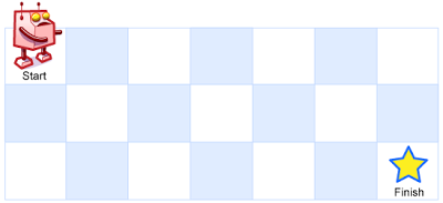
There is a robot on an m x n grid. The robot is initially located at the top-left corner (i.e., grid[0][0]). The robot tries to move to the bottom-right corner (i.e., grid[m - 1][n - 1]). The robot can only move either down or right at any point in time.

Given the two integers m and n, return the number of possible unique paths that the robot can take to reach the bottom-right corner.

The test cases are generated so that the answer will be less than or equal to 2 * 109.

Examples

Example 1:

Input: m = 3, n = 7 Output: 28

Example 2:

Input: m = 3, n = 2 Output: 3 Explanation: From the top-left corner, there are a total of 3 ways to reach the bottom-right corner:

1. Right -> Down -> Down
2. Down -> Down -> Right
3. Down -> Right -> Down

Constraints

• 1 <= m, n <= 100

Solving

This is a classic problem with many real-world applications, such as finding the shortest path in a maze or optimizing routes in logistics. In this blog post, we’ll explore how to tackle such grid problems using recursion and dynamic programming.

Intuition

Imagine we are on a grid with “rows” and “columns.” We always begin at the cell (0,0) and have two choices at each step: move right or move down. If you move right, the grid shrinks to (m, n-1), as you can’t go back to the left. Similarly, moving down reduces the grid to (m-1, n).

The Recursive Approach

Let’s consider a grid of size m * n. Instead of starting at the beginning, we’ll begin at the end cell, (m, n), and work our way back to (1, 1). In this reversed journey, our options are either to go up or to go left. At each step, the grid gets smaller, creating a smaller version of the original problem. This is where recursion comes into play.

Example: A 4x5 Grid

Imagine we have a 4x5 grid, and we start at the end cell (4, 5). We want to reach cell (1, 1). Here’s how we can break it down:

1. From (4, 5), we can either go left to (4, 4) or go up to (3, 5).
2. If we choose to go left to (4, 4), we are left with a 4x4 grid and can further explore options from there.
3. If we go up to (3, 5), we are left with a 3x5 grid and continue our journey.

By repeating these steps, we eventually reach (1, 1). However, there’s a catch. When we take longer paths, we may revisit certain cells multiple times. For instance, look into the following paths -

• (4,5) -> (4,4) -> (3,4) -> (2,4)
• (4,5) -> (3,5) -> (2,5) -> (2,4)
• (4,5) -> (3,5) -> (3,4) -> (2,4)

In these steps, we revisit (3, 4) and (3, 5) multiple times. As the path becomes more complex, revisiting cells becomes more common. This is where dynamic programming (DP) comes to our rescue.

Dynamic Programming to the Rescue

Dynamic programming allows us to optimize our approach by storing the results of subproblems we’ve already solved. In the grid problem, this means we don’t need to recalculate the number of ways to reach a particular cell every time. Instead, we can store this information and use it when needed.

For example, if we’ve already figured out the number of ways to reach cell (3, 4) in a previous step, we can reuse that information instead of recomputing it every time we pass through that cell. This significantly reduces the computational load for larger grids and complex paths.

Implementation

An implementation in python is shown below:

class Solution:
    memo = {}

    def uniquePaths(self, m: int, n: int) -> int:
        if m==1 and n==1:
            return 1
        
        if min(m, n) <= 0:
            return 0
        
        
        if (m,n) in self.memo:
            return self.memo[(m,n)]
        
        count = self.uniquePaths(m-1, n) + self.uniquePaths(m, n-1)
        self.memo[(m,n)] = self.memo[(n,m)] = count
        
        return count

In conclusion, solving grid problems using recursion and dynamic programming can be a powerful technique. By starting from the end and working our way back, we can efficiently find solutions while avoiding unnecessary recalculations. So, next time you encounter a grid puzzle, remember this approach - it might just make your journey a whole lot smoother!